The goal of this assignment is to learn about image filtering techinques through a few sub-assigments, among which are blurring images, sharpening images, creating hybrid images, and creating blended images.
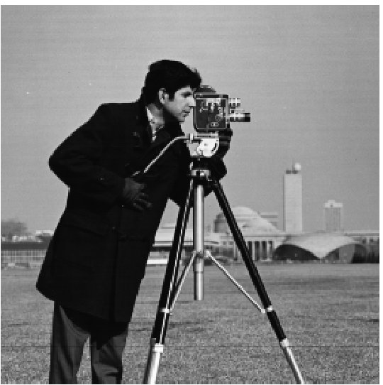
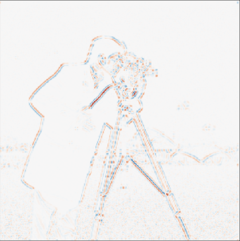
Given simple 2-d vectors Dx = [-1, 1] and Dy = [[-1], [1]], I convolved them with an image of a cameraman to take the partial derivative of the images with respect to these vectors. By highlighting the places in the image that corresponded to high derivative values, I was able to see where there was a high rate of change in the image with respect to the vector. Finally, I combined these values into a single edge image by calculating the magnitude of the gradient for each pixel.

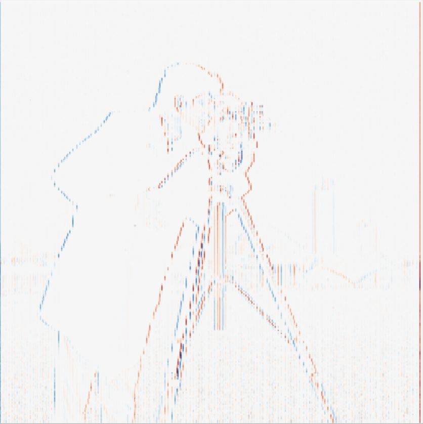
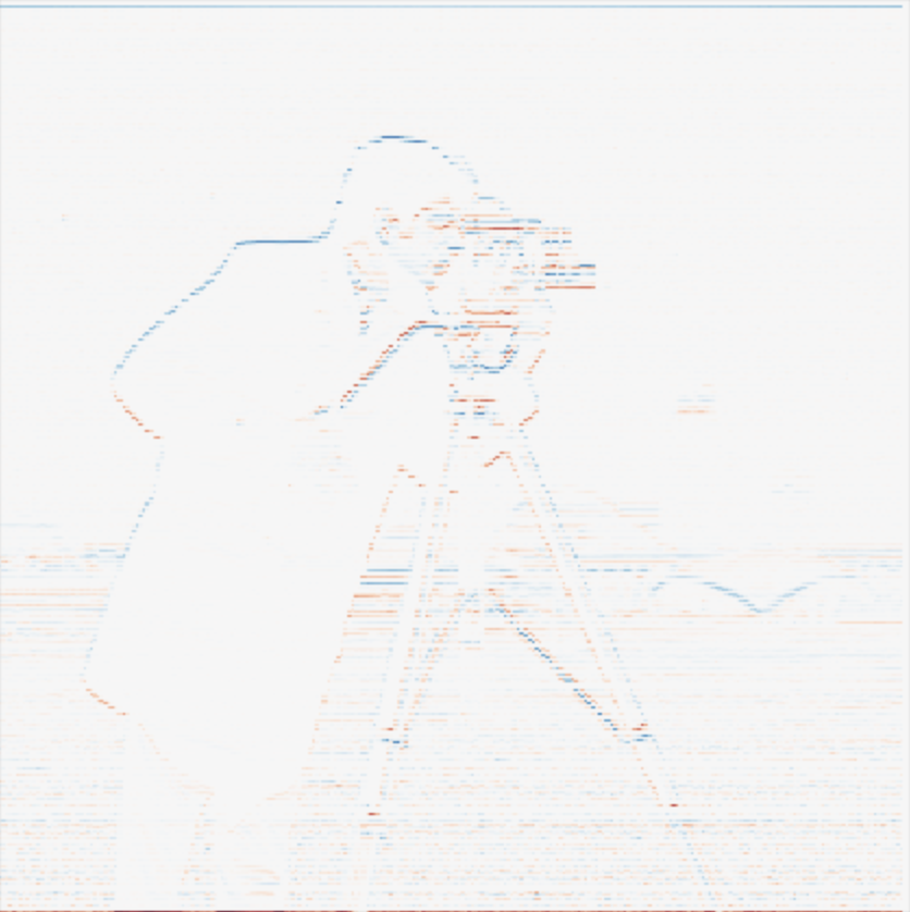
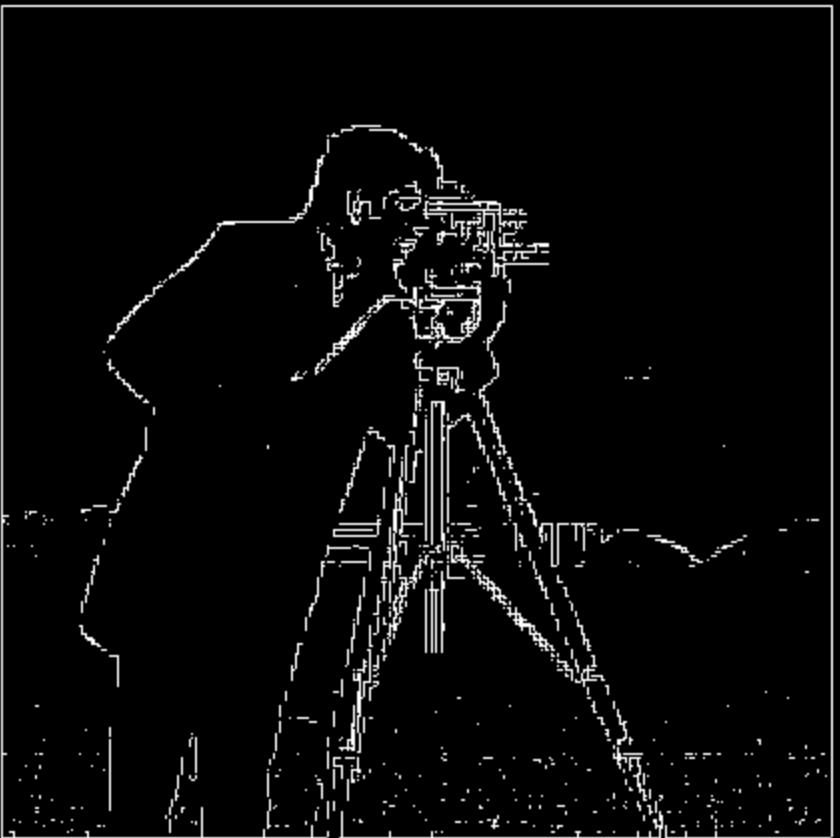
Because of the noise in the image, the edge readings were also correspondingly noisy. To combat this, I used a Gaussian filter to smooth the image and remove the noise, and along with that I performed edge computation. When I did this, I noticed less noise in the background of the image, particularly in the lawn underneath the cameraman. Also, because I used convolution for the filter and for edge computation and convolution is commutative, I was able to get the same result whether I smoothed the image and took the edges of that or if I convolved the gaussian first before using to smooth.
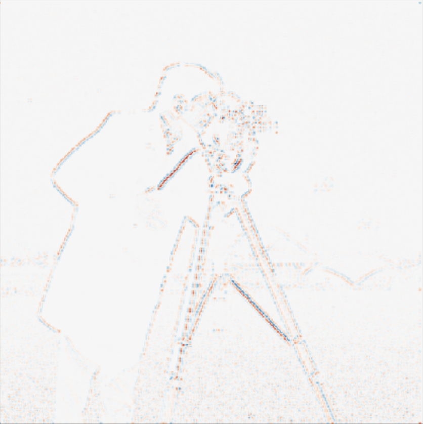
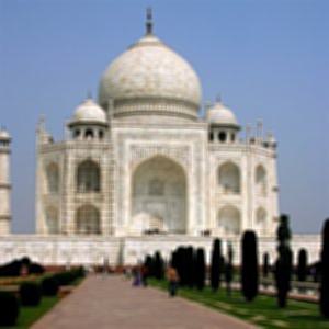
To sharpen an image, I first convolved it with a Gaussian filter to remove high frequencies. Then I subtracted the filtered image from the orignal to get just the high frequencies, and added the frequencies on top of the orignal image. Using the same technique, I also could resharpen blurred images.


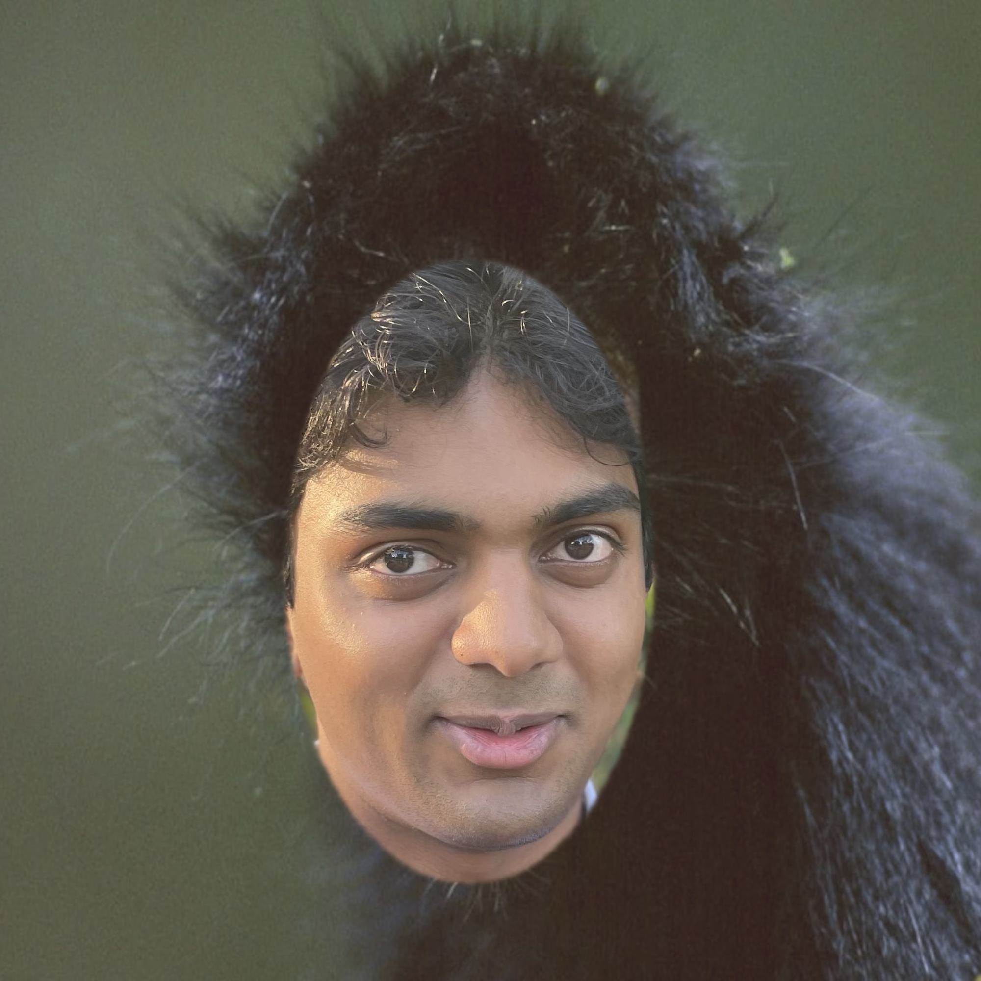
Hybrid images are static images that change in interpretation as a function of the viewing distance. The basic idea is that high frequency tends to dominate perception when it is available, but, at a distance, only the low frequency part of the signal can be seen. I blended high frequency and low frequency images into a single static image to try to achieve this affect, and some attempts were more successful than others.
I chose to take the more challenging route by using colored images and filtering them instead of simply using grayscale image, and this proved difficult because filtering colored images as much as I needed to create this effect distorted them to the point where they were hardly recognizable. I felt that neither the high or low frequency images were great at avoiding this effect, and I wasn't able to tweak my inputs for it to come out looking great.
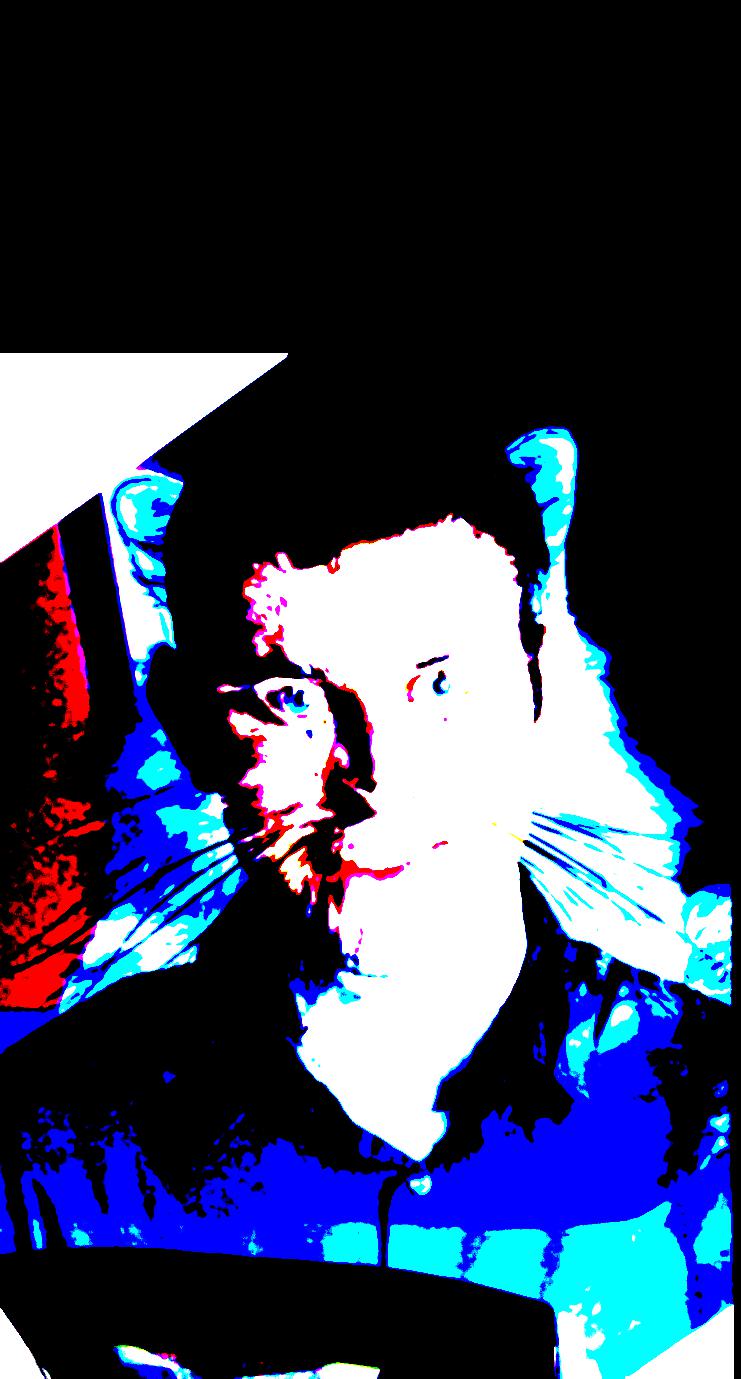
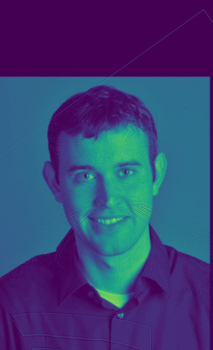
I tried some other images, but I still struggled to get the same effect as in the paper. I think it really came down to choosing good images that have similar enough characteristics to blend into each other nicely without
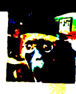
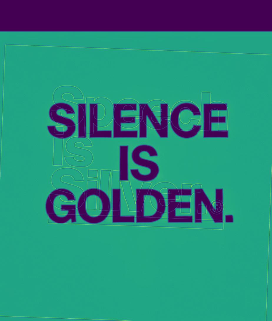
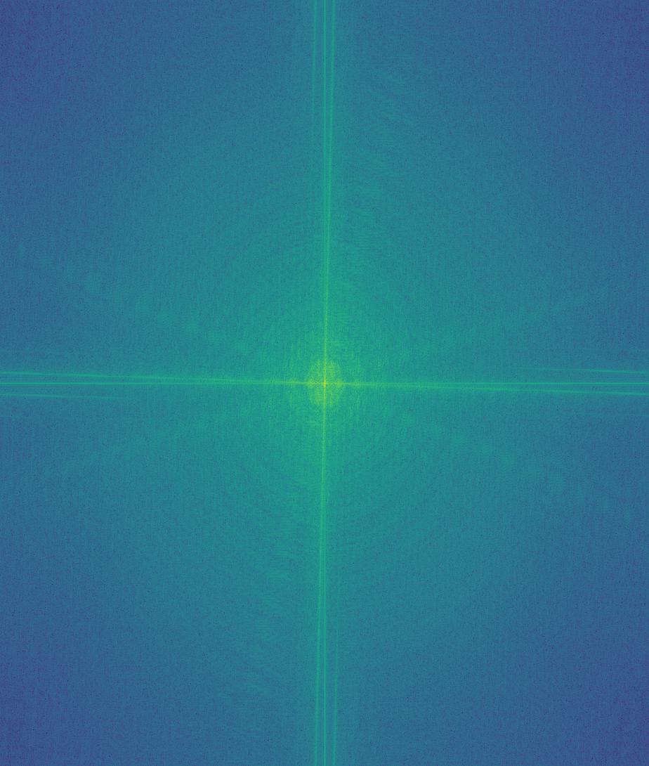
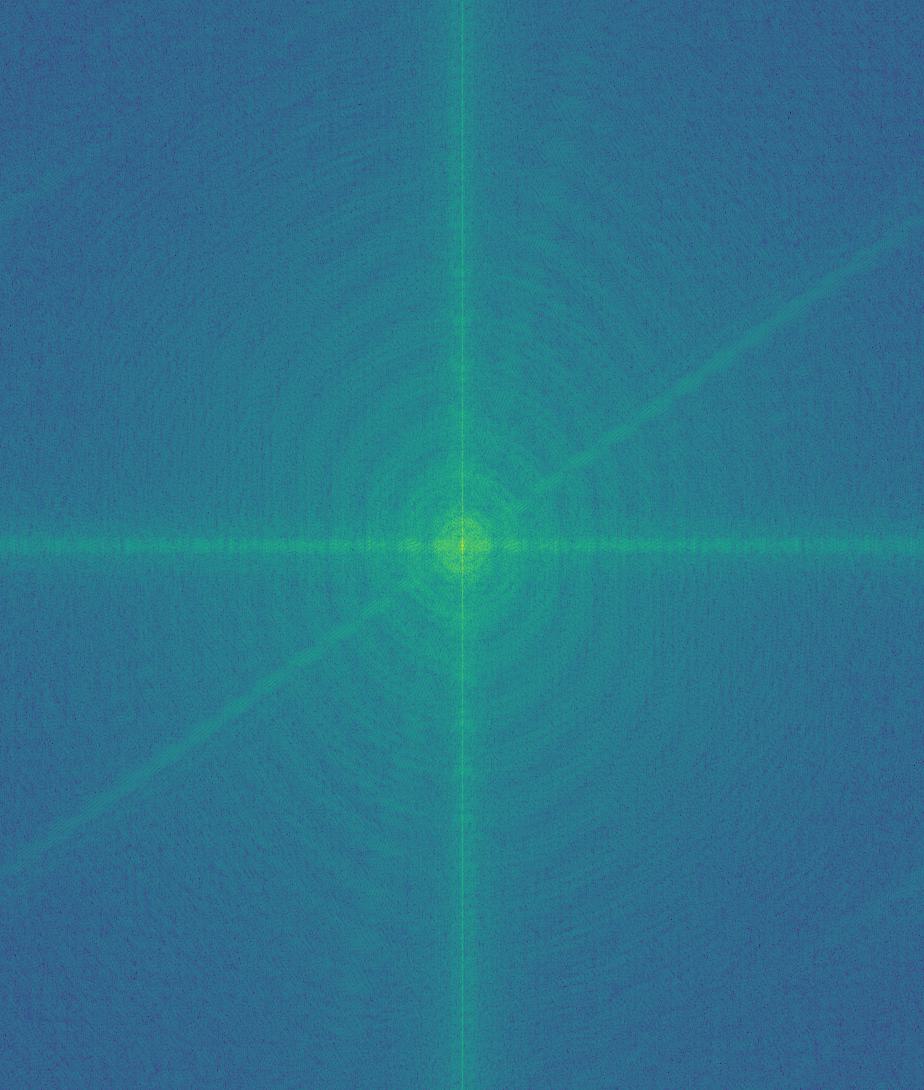
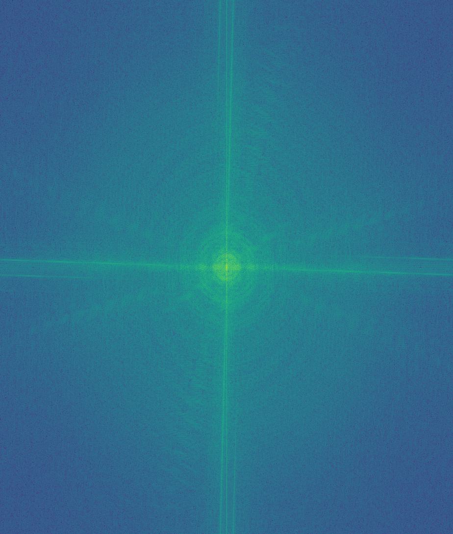
For my "Speech is silver, but silence is golden" image, here are the corresponding FFT graphs.
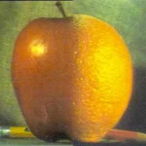
Finally, I used frequency manipulation to blend images. To do this, I created Gaussian and Laplacian stacks of images and a mask with the following method. For each level of the Gaussian stack, the previous level is blurred using a Gaussian kernel to get to the next level. The difference between successive images in this stack make up the Laplacian stack. Finally, the last blurred image in the Gaussian stack is added to the Laplacian stack. This way, the original image could be reconstructed by adding together all the images in the Laplacian stack.
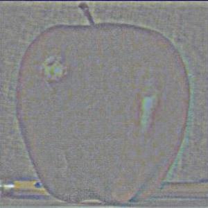
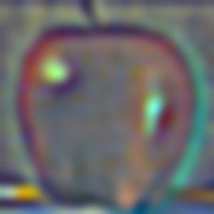
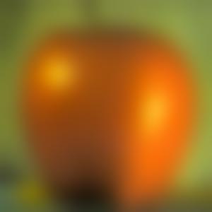
For the apple and orange, here are their laplacians at the 0th, 4th, and 9th indices.
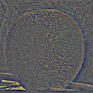
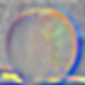
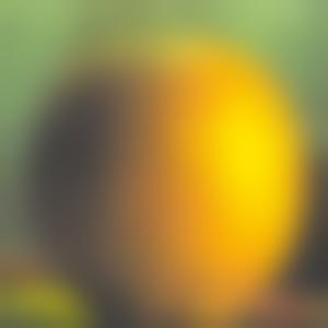
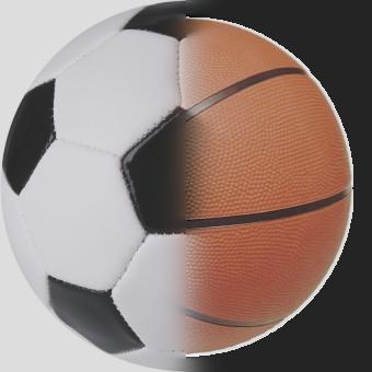
Finally, I used a mask to choose how to apply the amounts of each of the image to each other in my blended result. I created a Gaussian stack of my mask and for each level i in the stacks, I would multiply the mask with the corresponding Laplacian for the first image and the inverse of the mask for the second image. Here are the results. Hope you enjoyed.
